Module 1

 Introduction and Review

Section 1.3

 Equations and Inequalities

 (see Text Sections 1.4 and 1.6)

 

Introduction

 

An equation is just a statement that two expressions represent the same number or “value”. It may be always false, like 2=4 or , or always true like  or , or true for just some particular values of the variables like  

(which is true just for  ), or  (which is true for  ).

 

(An inequality is similar except that one of the expressions may be required to be greater than or less than the other.)

 

In practical situations we often want to find the values of some quantity for which something related to it has a given value or is within a given range. (e.g. to find the amount of fuel needed in order to travel a given distance). Such problems are often solved by writing the condition as an equation or inequality and then solving for the required variable.

Your objectives for this section are to recall and demonstrate facility with equations and inequalities.

 

Study Notes and Discussion

 

Equations

 

Solving an equation for a variable v means finding all values of that variable for which the equation is true. If there are other variables in the equation, then the solution may have to be expressed in terms of them rather than just as a specific number. This amounts to writing the equation in the form of v = expression where v does not occur in the expression on the right hand side. (For example, in the equation , we can solve for v in terms of b by subtracting b from both sides to get .)

 

Note that the variable we are solving for does not have to be called x. But if there are several variables, the one required will be specified. So for example one might be asked to solve for b in the equation . (see answer #1)

 

The terms and techniques in section 1.4 should all be review, but now is a good time to point out that your solutions to problems should be as complete and clearly written as those in the book’s examples. Don’t just follow procedures but, for each statement you write down, think about what it means and why it is true rather than just whether it follows a pattern you remember.

 

The procedure used to prove the quadratic formula on page 54 is called “completing the square” and it can be useful practice to apply it in problems as an alternative to just plugging into the formula.

 

 For example in the text’s Example 5 on page 55, we have the equation . Dividing  by 2 gives , or . Now , and if we take  then the first two terms match the left side of our equation. So if we add  to both sides, then we will have ,  or in other words . So .   So .

Can you do the same for Example 7 on page 57 of the text? (see answer #2)

 

 

 

Inequalities and Interval Notation

 

Just as the goal of solving an equation for a variable v is to express it in the form

v = expression, so for inequalities our goal is to get a simplified form of the given statements in terms of  simple bounds on the variable v itself.

 

A pair of simple bounds like  and  confines v to an interval on the number line and the interval notation described at the beginning of the text’s section 1.6 is an important tool for describing the solution sets of inequalities.

 

It is important to distinguish between sets of conditions which must all apply and those for which just one may apply  i.e. between the use of ‘and’ and ‘or’ between the conditions. For example the condition ‘  and  ’ confines v to an interval, but the condition ‘  or  ’ is satisfied by any real number. Notice that the use of ‘and’  between conditions does not give more solutions but rather fewer. In fact, it describes a smaller set consisting of the overlap or intersection of the sets described by the two conditions separately. At this point you might want to look back at the discussion of set notation at the beginning of the text’s section 1.3 and try expressing the above discussion in terms of the curly brackets notation described on page 32. (see answer #3)

 

 

If an inequality has zero on one side, then it can be solved just by checking the sign of the other side. The properties of multiplication of signed numbers allow us to do this by factoring  as shown in the text’s Examples 7 through 11 in section 1.6.

 

Note: Just as for solving equations by factoring, it is essential that one side be zero.

 

When there are several factors to consider, the easiest way to keep track of them is with a table or chart. The book shows two alternatives but the graphical one has the advantage that you don’t need to know the intervals to start with. Perhaps it would be better to draw it the other way up though  with the number line at the top, then the sign information for each factor, and finally the resulting sign at the bottom.

 

Doing the text’s Example 9 this way, and including all the factors and their powers gives the following picture

 

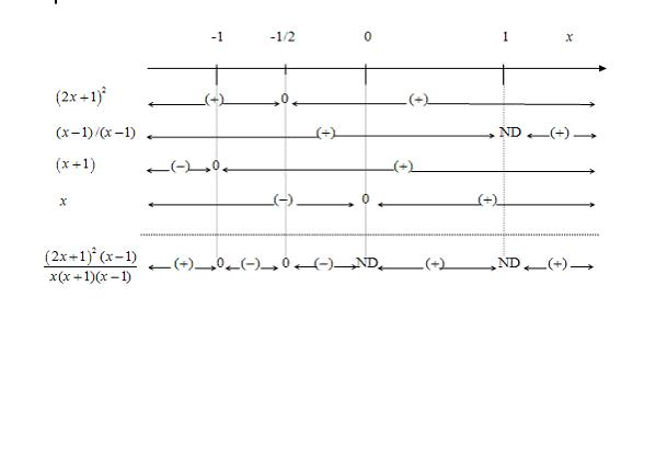
(Here we are using ND to denote “not defined”)

 

 

Further Practice

 

Check your understanding and practice for speed by working through some of the Exercises on pages 61-67 and 85-87

 

 

Do enough of the odd numbered questions of each type to convince yourself that you can get the right answers. (Note that, as usual, the answers are in the back of the text and complete worked solutions are in the student study guide - but try to avoid looking at answers or solutions until you have made your own best effort)

 

As a minimum you should do ##1,5,11,15,21,35,41,45,51,55,61,65,71,75,83 and 87 from Section 1.4 and ##1,5,11,15,21,35,41,45,51,55 and 61 from Section 1.6.

 

 

 

 

Optional Reading

If you are finding things a bit too easy you may want to read section 1.5 of the Text and learn about how the Real Number System can be extended to include solutions of quadratic equations even when the discriminant is negative. This can be done by including algebraic combinations of real numbers with an imaginary unit whose square is -1 to get what is called the “Complex Number System”. Since the squares of positive and negative numbers both have to be positive, this extended system must include numbers which are neither positive nor negative. Such complex numbers are algebraically useful but cannot be represented by points on a single line so do not correspond to simple physical measurements. Since the focus of first year calculus is on relationships between measurable quantities, you will not actually need to know about complex numbers in your calculus courses and so will not be required to study them in this course.