Module 3 

3.2
(see Text section 3.1)
Introduction
In this section we go beyond the linear and quadratic cases that we studied in section 3.1 to study also functions involving higher powers of the variable.
Among the practice problems from section 2.6
of the text, you saw examples in which quadratic functions were used to
describe areas not surprising since the area of a rectangle
is obtained by multiplying two lengths. But the volume of a box is the product
of three lengths (or the cube of the
side length if they are all equal), so volume problems often lead to functions
involving the third power
also known as cubic functions. All three cases of linear, quadratic and cubic
functions are included in the larger class of polynomials which comprises all sums of whole number powers of the
variable.
This class of functions is the topic of the current section.
Definition
The general polynomial is a function of the
form .(Here
we are using the same letter c with
various subscripts to represent the different numerical coefficients rather than trying to come up with enough letters to
use a different one for each.) The
highest power occurring with nonzero coefficient is called the degree of p.
Graphing Polynomials
Perhaps the most important fact about
polynomial functions is their behaviour for large values of the argument (independent
variable). This behaviour is determined by the highest power term because for
large enough values of the variable that term will be much larger than all of
the rest. E.g. for ,
the
term will be bigger whenever
.
(Note: The most significant term is often called the “leading term”, but
despite its name, the “leading term” does not always have to be written first,
though by convention it usually is.)
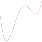
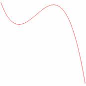
In general, if the degree of p is
even, then the graph of p will have the same behaviour at both
ends (that is, either with the graph going up at both ends, or
which means that it goes down at both ends).
OR
Even degree graphs
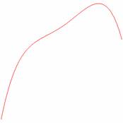
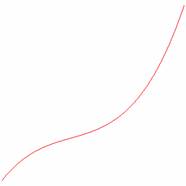
On the other hand, if the degree is odd then
the graph will go up at one end and down at the other (that is, either ,
as in the graph on the left below, or
).
OR
Odd degree graphs
Q1
In either case, since the powers can all be
calculated for any real value of x,
the domain of p(x) is all reals. Also, if we make a small enough change in x, then the corresponding change in p(x)
will also be small. So the points on the graph should all be joined together
without any jumps or gaps. (This is the property that will be called
“continuity” in your calculus course.) So if we know the values of p(x)
for two given x values, then it must
pass through every value between them. This is called the “Intermediate Value
Property”. How does this guarantee that any odd degree polynomial must have at
least one real root?(see answer #1)
Once we have determined how the graph goes
as (ie at the far right and far left) we need to
figure out what happens in between.
To see how the graph behaves in the middle region we can start by looking for intercepts.
The y-intercept
is easy. It is just equal to the value of the constant term, .
For x-intercepts
we need to solve an equation which is not
always easy. In fact, unlike the quadratic case, there is no general formula when
. But, what does work just as for quadratics, is
that if we are given or can find a factorization of p, then this will help us to find solutions of the equation
.
If a factor of form occurs in
,
then
and the graph has an x-intercept at
.
In that case we say r is a root of p . If the factor occurs with a power m we call m the multiplicity of the root, and say that r is a root of multiplicity m.
Once we have located all the x-intercepts, we can check signs in between to get an idea of the shape of the graph. We can do this either by substituting test values, or just by checking the signs of the factors in a “sign chart” as in Examples #3&4 of the text.
Q2
For a root of even multiplicity for p, there is no overall sign change of
the function
at the root, and the graph just touches the x-axis without crossing. But at a root
of odd multiplicity there will be a sign change, and the graph will cross the x-axis at that point. These facts can be
used to shortcut the sign chart process
try using this approach to show that the signs
of
are as shown in Example#5 on page 212 of the
text (see answer #2).
For these ideas to be useful, we need to be able to factor the polynomial. It would be a good idea at this point to recall some of the most useful factoring techniques.
Factoring Polynomials
- Common Factor: The most obvious is extracting a common factor. This is easy to do if there is a monomial (single term) which divides into all of the terms in the polynomial.
eg .
Is this factorization complete? (answer#3)
- Grouping: Sometimes it is possible to divide up the terms into groups so that all of the groups have a more complicated common factor.
eg
- Difference of
Squares: Using
eg
- Completing Squares:
eg
- Difference and Sum of
Cubes: Using
eg
- Recognizing Higher Powers of Binomials: Using Pascal’s Triangle
eg
- Substitution of Powers: Using the ‘power of power’ rule for exponents
eg
- Trial Division: This is just like what we often do when factoring numbers.
eg To factor 299
we might try dividing it by successively higher numbers until we find that the
division by 13 does work out exactly (with zero remainder) and gives .
We will be able to do the same sort of thing with polynomials after reviewing
how the “long division” algorithm of arithmetic can be extended to work also
for polynomials. This will be the topic of the next unit.
Further Practice
Check your understanding and practice for speed by working through some of the Exercises on pp.215-219
Do enough of the odd numbered questions of each type to convince yourself that you can get the right answers. As a minimum do at least ##3,7,15,25,29,35,39,41 and 45.